Data Science

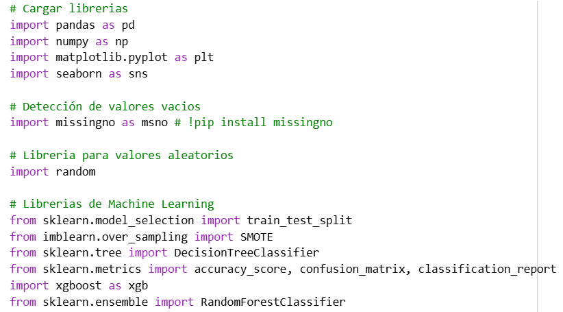
We need to import well-known libraries such as: pandas, numpy, matplotlib, seaborn, missingno, random, sklearn, imblearn, and xgboost.

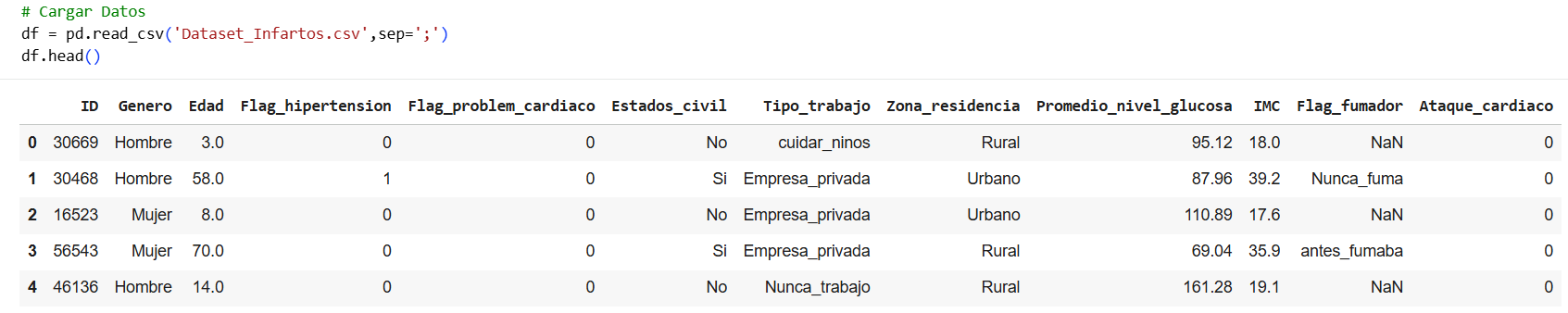
We use our Excel database to see which columns it has and begin our study.

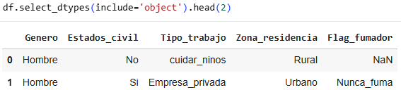
In this case, we can see the columns in our dataset, always showing the first five columns. We can see from the outset that most columns have corresponding values, although in the Flag_smoker column there are empty values or NaN. It is necessary to clean up the data, either by checking the number of NaN values that exist.

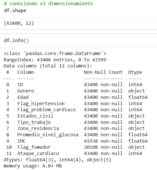
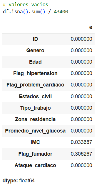
Here we see the number of rows in each column and we see that most have 43,400 data points. However, for the BMI column we see that it has 1,462 null data points and Flag_smoker has 13,292 null data points, which equates to 3.4% and 30.6% respectively.

From here, we can make our first analysis regarding these two columns. We say that “if the percentage value is less than 10% or 15% maximum, an imputation can be made for the values, for example for BMI, and if it is higher, the variable is eliminated, for example for Flag_smoker.”

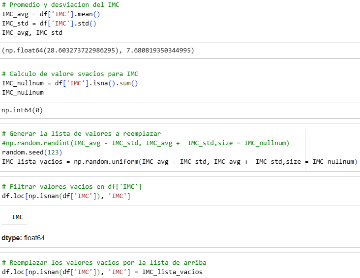
We have to compare the mean and the standard deviation, verify that the mean is greater than the standard deviation. In the case of Flag_Hypertension-Flag_Heart_Problem, we see that they are 0 and 1.

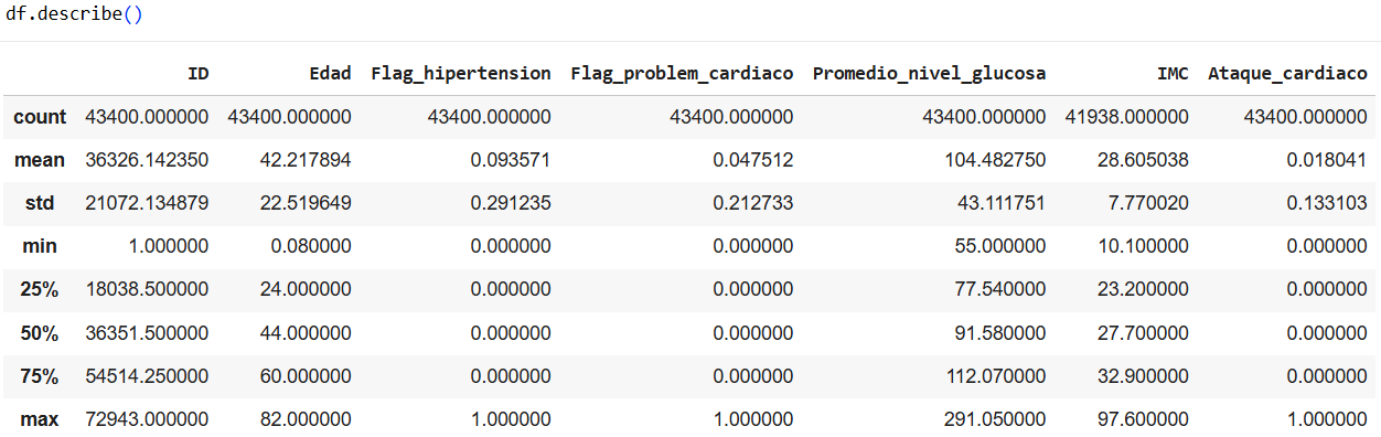
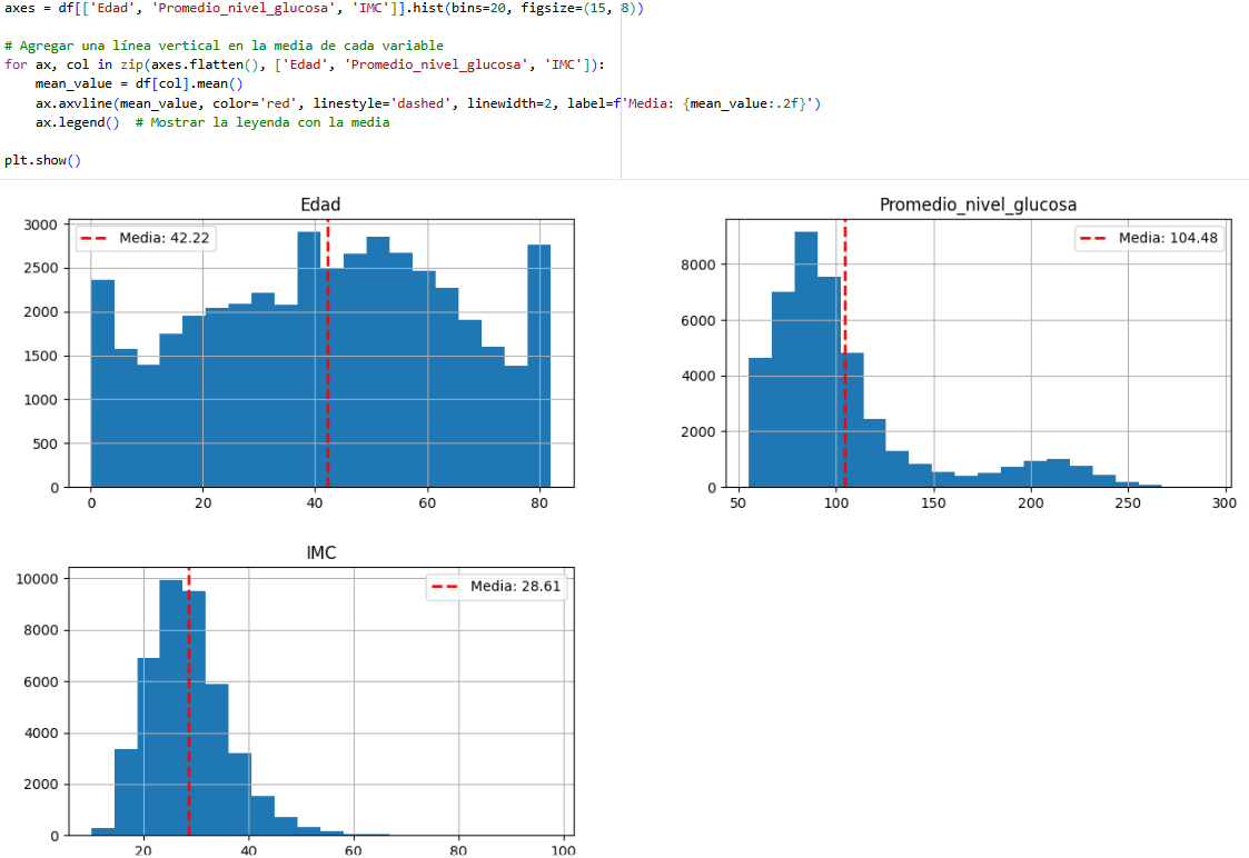
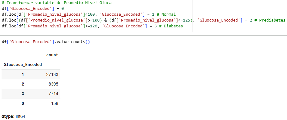
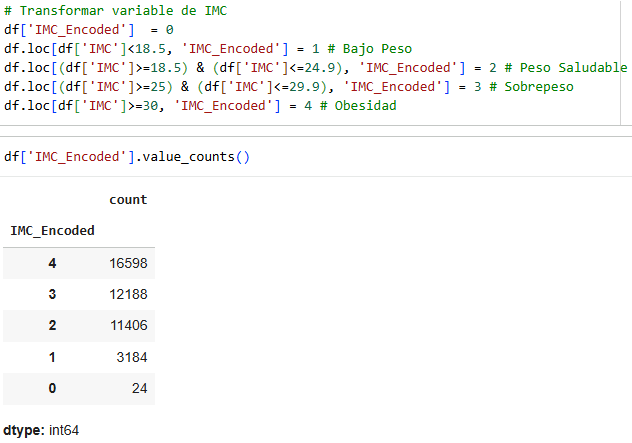
By knowing each of the averages, we can see where the corresponding values are grouped most. As we saw in class, glucose levels are very important for identifying whether someone is diabetic. Less than 100 mg/dL is considered normal. Between 100 and 125 or more in two different tests is diagnosed as diabetes. On the other hand, the age range between 40 and 60 years old is where the most data is stored. When looking at the body mass index, we can see that it is used to identify weight categories that can lead to health problems. If we had an extra variable such as height, we could calculate the appropriate BMI for each person, but we see that the data is between 20 and 35.

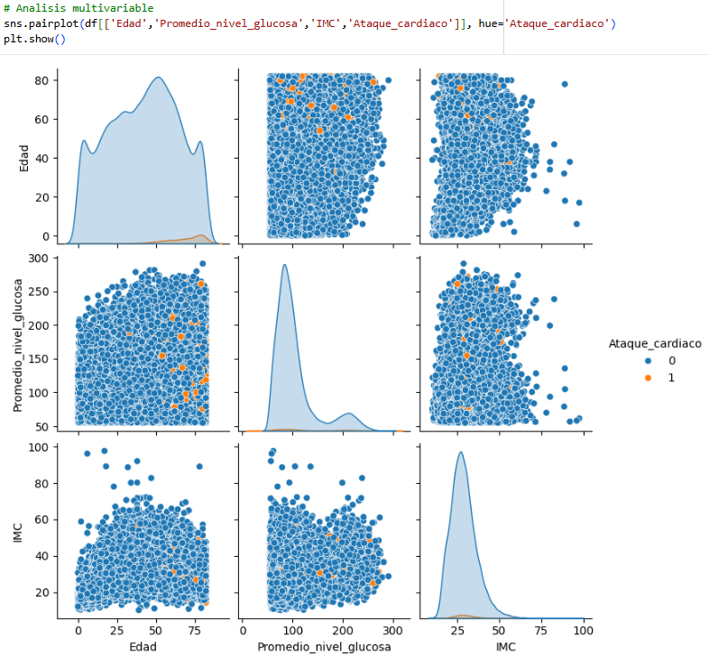
In Age and IMC, we see that heart attacks are directed toward a specific group, usually adults and people with levels between 22 and 35. If we compare the other variables, the only one where we can see significant information is the relationship between age and glucose level, where it is very clear that heart attacks affect adults more, regardless of their glucose level. We can also see IMC vs. glucose level. We see that the orange dots are distributed throughout the diagram, but we can see a straight line where heart attacks are frequent if the BMI is greater than 25.

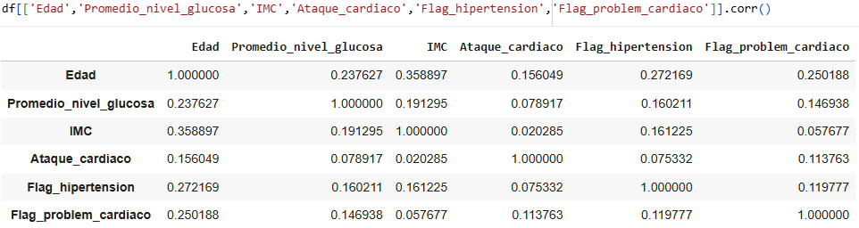
Here we can review the correlation for heart attack, which is our target. We must always bear in mind that the closer it is to 1, the greater its correlation. Therefore, the most important variables are age, glucose level, and IMC.

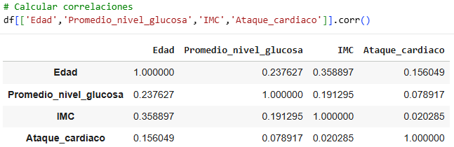
Here we can see the same thing as above, only with more variables, and if we want to choose only three important variables, they would be the ones we have in the previous code.

To make a decision on whether a variable is relevant or significant, we look at the measurement of each variable with respect to heart attacks. For large volumes of data, if the percentage increase is greater than 5%, we can say that the variable is relevant. Conversely, if the volume of data is much smaller, we look for it to be higher than that 5%, ideally around 10%.

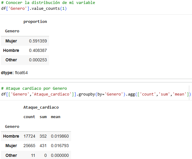
Bearing in mind that the proportion of heart attacks is 1.8%, we compare gender and see that the proportion that increased was only 0.1%, so gender is not relevant in determining whether or not someone will have a heart attack.

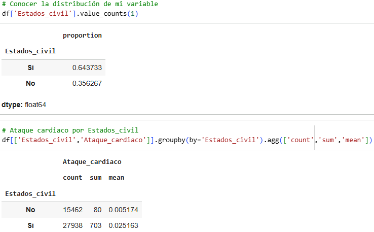
Bearing in mind that the proportion of heart attacks is 1.8%, we compare marital status and see that the proportion that rose was 0.7122%, equivalent to 39.5%, so marital status can be a relevant variable in determining whether or not someone has a heart attack. In conclusion, married people are more likely to have heart attacks.

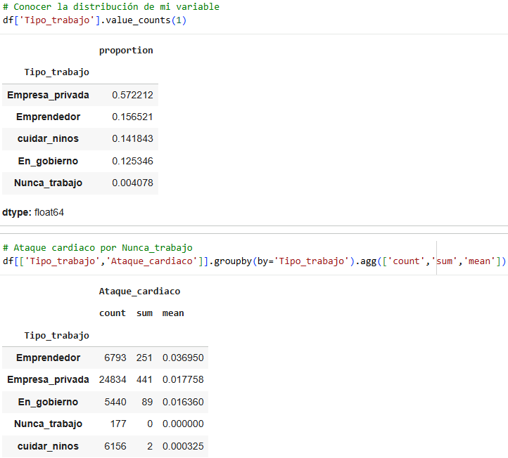
If we follow the same order, the type of work is a significant variable, as we can see that for entrepreneurs, the average is high, exceeding the proportion of heart attacks. The other jobs remain the same except for Never works and Childcare.

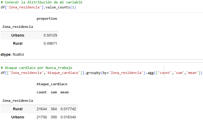
For the variable “area of residence,” we see that the average does not change; therefore, it is a variable that does not have much influence when it comes to determining whether it causes heart attacks.

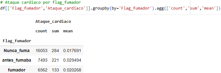
We see that this smoker flag variable contains a lot of empty data, so we don't know how this variable might be behaving.

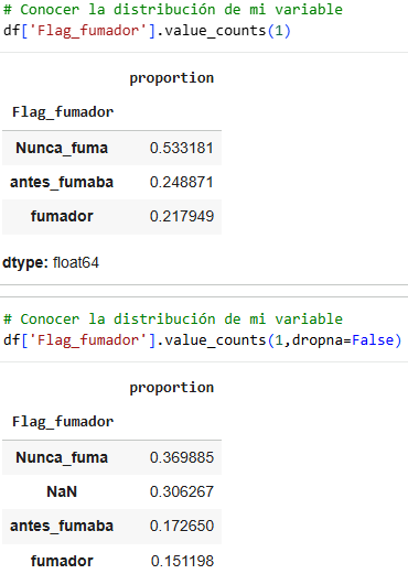
If we want to use the smoker flag variable, what we could do is create a separate column where we put 1 and 0, 1 is used if data is found in the smoker flag variable and 0 if it is null.

As indicated in class, the important variables would be:

Numerical variables: Age, Heart_problem_flag, Average_glucose_level, Hypertension_flag and IMC

Important qualitative variables: Marital_status and Type_of_work

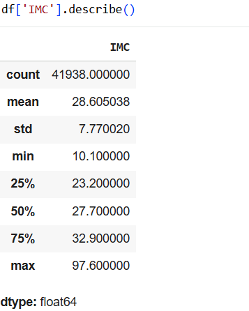
As we saw from the outset, the BMI variable has missing values: 1,462 null data points, equivalent to 3.4%. Therefore, we can use the most efficient imputation method, which is confidence intervals, to complete the null values.

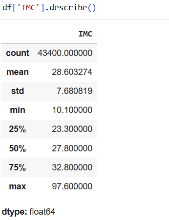
We can now see that our missing data has been completed.

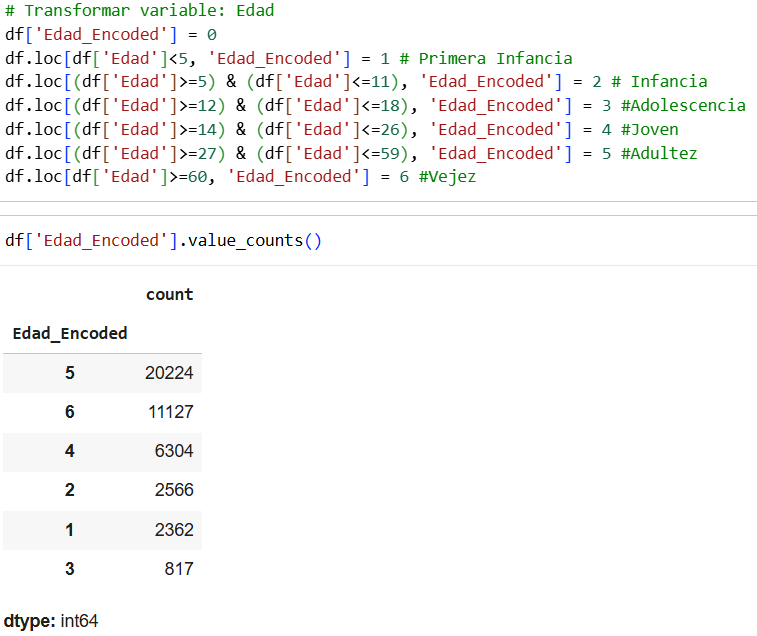
It is interesting in some other exercises to apply the following classification of generations.

We transformed the average glucamine level variable according to the following classifications.

We transformed the BMI variable according to the following classifications.

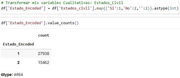
Indicate whether the marital status variable says yes, then enter 1; if it says no, enter 2; and if it is empty, enter 2.

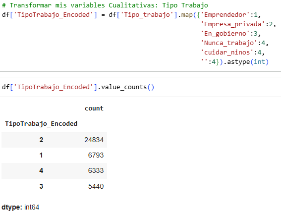
We transform the work variable according to the following classifications.

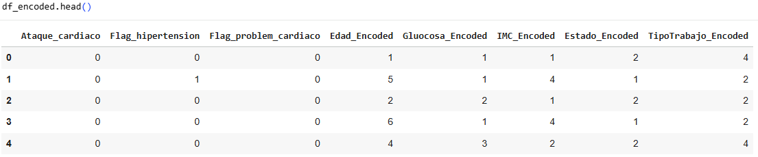
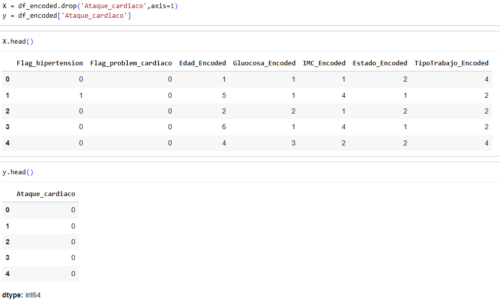
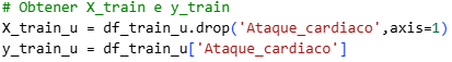
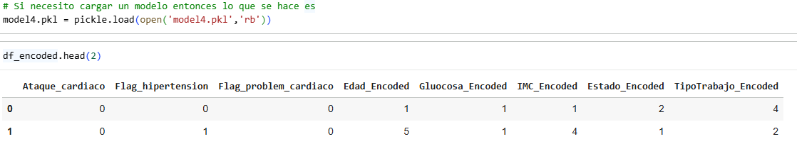
We select the variables we will use and save them in a new table.

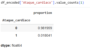
Our data is unbalanced, with either 0 being the majority number and 1 being the minority number.

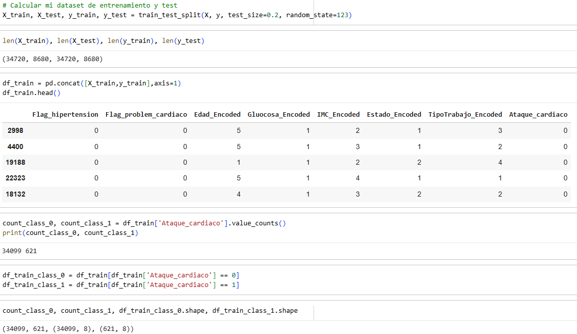
We have three balancing methods: 1. UnderSampling, 2. OverSampling and 3. SMOOTE

We will see how each of the methods performs in our dataset.

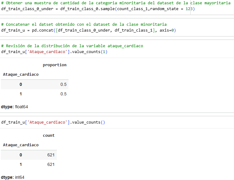
We will first use the UnderSampling method.

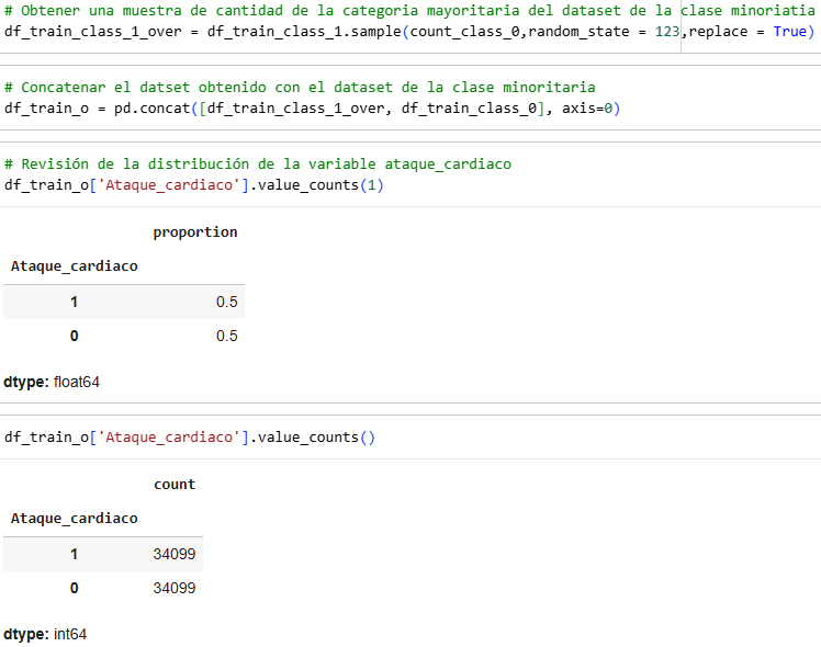
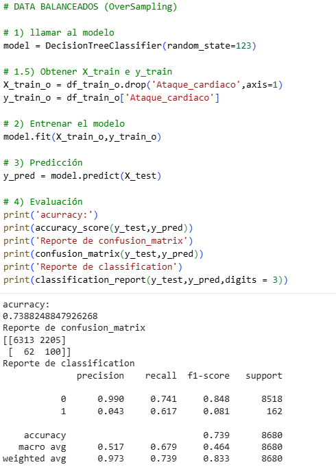
OverSampling works in the same way, only now it is done in reverse.

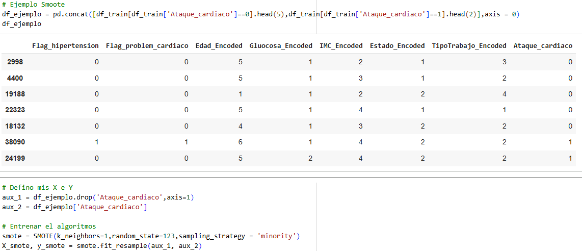
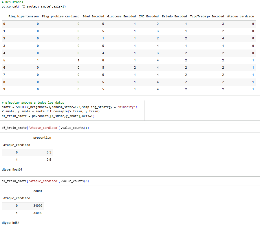
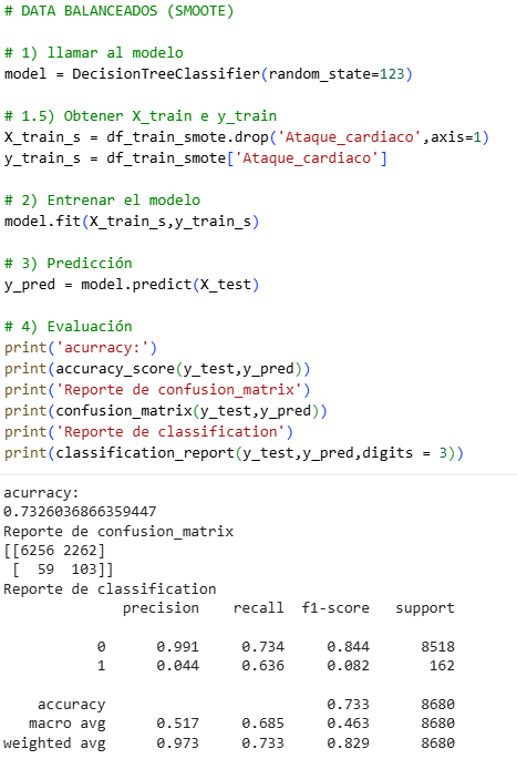
Finally, we will look at the SMOOTE method.

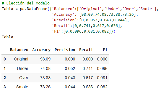
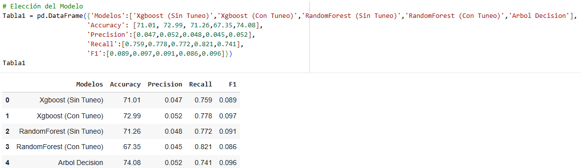
We already have the three models; now we need to decide which one to choose, which one will be the best of the three.

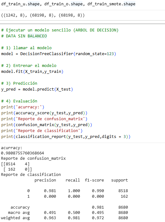
There is something wrong with the accuracy, which is 0 for our category 1. In the matrix, we see that it does not recognize any of the four data points that appear, so something is wrong. This is for our original data.

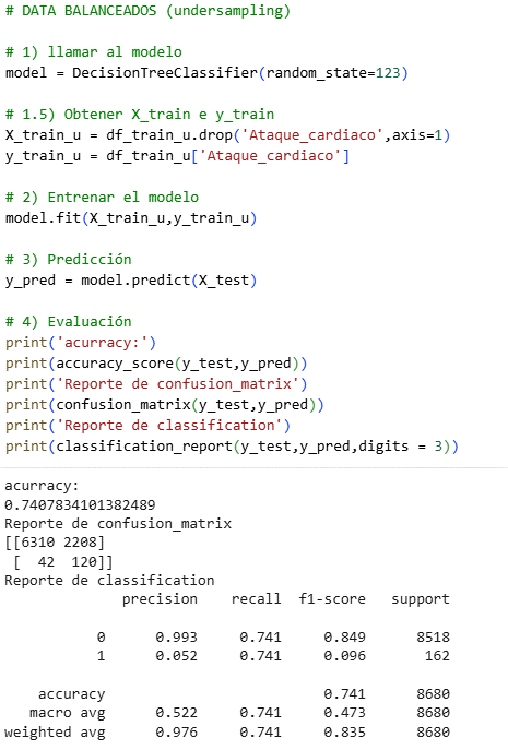
It is very interesting to analyze this data, since in some cases the Precision number is more important and in others the Recall number is more important. For this exercise, we will use Recall, since it is said that for the bank, sending many people with precision to heart attacks would be an economic expense, therefore Recall is better in this case. The best of all is undersampling with a Recall of 0.741. In other cases, such as house sales or calls, we could use Precision, and the choice would be the same undersampling.

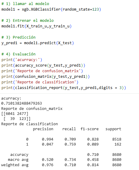
We begin with our decision trees using the method: Xgboost (Untuned).

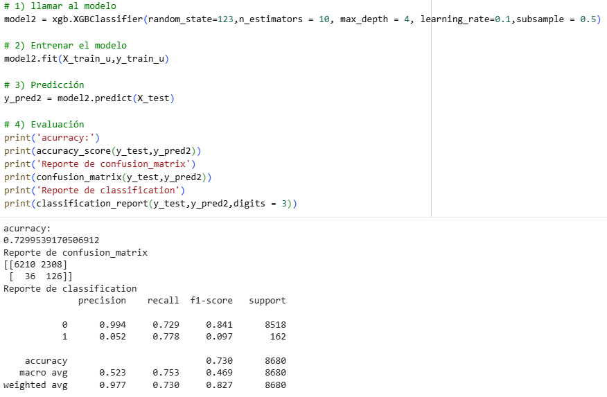
Xgboost method (Tuned)

Random Forest Method (Unmodified)

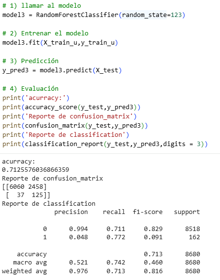
Random Forest Method (Tuned)

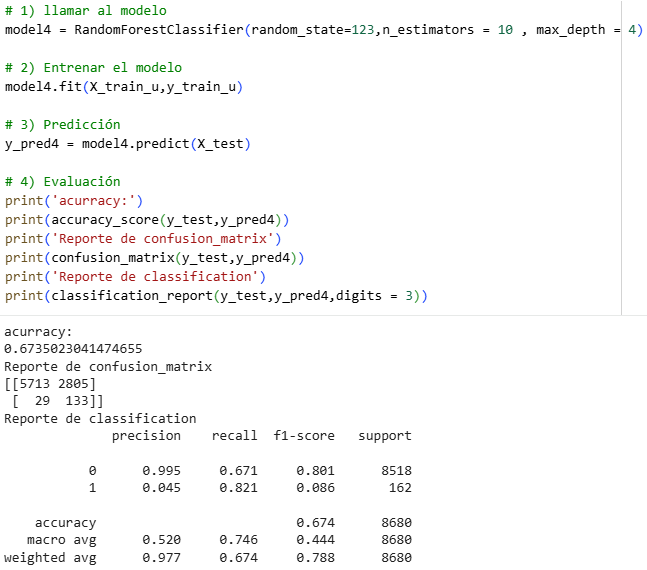
To choose the best model, we can review Recall again and see that RandomForest with tuning has the highest value of all, which is the best option for our model. If the RandomForest method (with tuning) were not used, as in Recall we see very similar numbers, we would have to look at other columns such as Accuracy, and the one with the best Accuracy is Xgboost. (with tuning).

On the other hand, if we end up with a larger volume of data, Xgboost may work much better, whereas for RandomForest, a smaller amount usually works better.

If I want to work on another computer, what I do is.

Export the model that works for us and appears in our folders.

If I need to load a model, then what I do is.

We define a set of fictitious data.

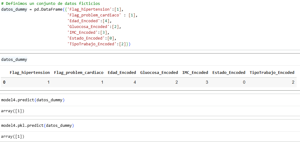
So, based on the data you entered in line 112, you are indicating that number 1 This means that they may have a heart attack, so the insurance company will not provide them with service or could possibly charge the customer more to reduce the loss of money. What can also be done is to offer policies with premiums adjusted to risk, suggest preventive health programs with incentives (discounts for lifestyle improvements), or create early detection programs in collaboration with medical institutions.

Download File.py